Tutorials

Here we’ll outline how use pauxy to calculate the imaginary time correlation function (ITCF) as well as various ground state estimates of the 3x3 Hubbard model with periodic boundary conditions.

The input file is given as follows:

{
    "model": {
        "name": "Hubbard",
        "t": 1.0,
        "U": 4,
        "nx": 3,
        "ny": 3,
        "ktwist": [0.01, -0.02],
        "nup": 3,
        "ndown": 3
    },
    "qmc_options": {
        "method": "CPMC",
        "dt": 0.05,
        "nsteps": 1000,
        "nmeasure": 10,
        "nwalkers": 30,
        "npop_control": 10,
        "rng_seed": 7
    },
    "trial_wavefunction": {
        "name": "free_electron"
    },
    "propagator": {
        "hubbard_stratonovich": "discrete"
    },
    "estimates": {
        "back_propagated": {
            "nback_prop": 40
        },
        "itcf": {
            "stable": true,
            "tmax": 2
        }
    }
}

Note that we added a small twist to lift the degeneracy in the free electron ground state, we’re using a free-electron trial wavefunction and that to calculate the ITCF we also need to set the back propagation time to be sufficiently large so that the left handed wavefunction is close to the ground state.

First we’ll run pauxy as follows:

$ python3 -u ~/path/to/pauxy/bin/pauxy input.json > 3x3.out

By default pauxy will print some basic information to stdout, including periodic estimates for mixed estimates of the energy. All estimates will also be saved (by default) to the estimates.0.h5 file.

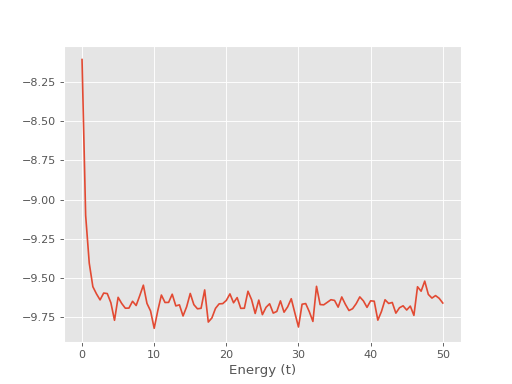
Once the calculation has finished we can inspect the output. It’s helpful to first plot the energy data from the 3x3.out to inspect when the simulation has equilibrated and to get a rough idea of the quality of the result.

(Source code, png, hires.png, pdf)

To be safe we’ll discard data before \(\tau t=10\) and analyse the data as follows:

$ ~/path/to/pauxy/tools/reblock.py -s 10 -f estimates.0.h5

which will analyse all the estimates in estimates.0.h5 and dump the results to a second file called analysed_estimates.h5. We can extract then extract the estimates by doing

$ ~/path/to/pauxy/tools/extract_observable.py -o 'energy' > basic.out

ndets    dt         E   E_error       EKin    EKin_error     EPot  EPot_error
  1.0  0.05 -9.667367  0.006009 -12.107177  8.560304e-16  2.43981    0.006009

which will extract the mixed estimates. For the back propagated estimates we can do

$ ~/path/to/pauxy/tools/extract_observable.py -o 'back_propagated' > back_propagated.out

to find

nbp    dt          E   E_error          T   T_error         V   V_error     weight  weight_error
40.0  0.05 -10.172595  0.221067 -11.445905  0.241082  1.273311  0.038141  30.376271      0.301327

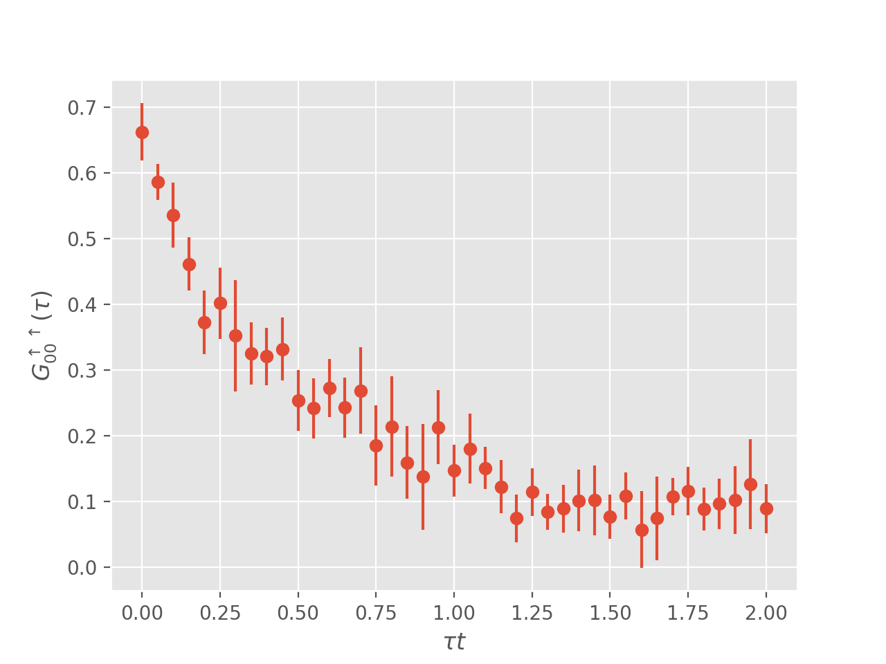
and finally the greater one-particle imaginary time green’s function as

$ ~/path/to/pauxy/tools/extract_observable.py -o 'itcf' -s up -t greater -e 0,0 -f analysed_observables.h5 > itcf.out

which we can then plot

(Source code, png, hires.png, pdf)

As you can see, the error bars are still quite large so you should run for longer.